 KELIBRON
 Tolerances and decisions
An uncertainty budget for a caliper measurement
An uncertainty budget lists every source of uncertainty, turns each into a standard uncertainty, combines them as the square root of the sum of squares and multiplies by a coverage factor. In NPL’s caliper example (resolution 0.02 mm, specification ±0.02 mm, five readings) the combined standard uncertainty is 0.017 mm (NPL writes 0.018) and the expanded uncertainty U = 0.035 mm for k = 2.
On this page
Which sources go into a caliper budget?
NPL Good Practice Guide 40 lists six for a caliper measurement: calibration errors that are not corrected (or only known to be within specification), flatness of the measuring faces, parallelism of the faces, squareness of the faces to the beam, resolution, and the random variation seen in repeated readings. Squareness either produces a cosine error small enough to ignore or shows up as a parallelism error, so it needs no separate line.
How is each source turned into a standard uncertainty?
The GUM gives three conversions that cover a caliper budget; the lines are then combined as a root sum of squares, which assumes they are independent and each affects the reading one for one:
- Repeated readings (Type A): the experimental standard deviation s of n readings; the standard uncertainty of their mean is s/√n.
- A limit ±a with any value inside equally likely (rectangular distribution, Type B): u = a/√3.
- Resolution δ of the indication: u = δ/√12 = 0.29δ.
Worked example: the NPL caliper budget
The caliper reads to 0.02 mm and is specified to ±0.02 mm; its faces are flat to 0.005 mm and parallel to within 0.008 mm. A part is measured five times: 20.08, 20.08, 20.06, 20.10 and 20.12 mm. The mean is 20.088 mm and s = 0.0228 mm. The calibration certificate says only that the caliper meets its specification.
| Source | Value | Conversion | Standard uncertainty |
|---|---|---|---|
| Repeatability | s = 0.0228 mm, n = 5 | s/√n | 0.0102 mm |
| Resolution | 0.02 mm | δ/√12 | 0.006 mm |
| Face flatness | 0.005 mm | a/√3 | 0.003 mm |
| Face parallelism | 0.008 mm | a/√3 | 0.005 mm |
| Within specification | ±0.02 mm | a/√3 | 0.012 mm |
Combining the unrounded lines gives uc = 0.0173 mm and U = 2 × 0.0173 = 0.035 mm, the value NPL reports. With the rounded figures in the table, uc = 0.0178 ≈ 0.018 mm. NPL treats the lines as independent; a stricter budget would check whether the specification line already covers part of the face and repeatability effects.
Do five readings change the coverage factor?
k = 2 assumes the standard uncertainty is well known. The repeatability line rests on only 5 − 1 = 4 degrees of freedom, and NPL notes that its simple calculation ignores this: for fewer than 10 readings the degrees of freedom should be taken into account, and it suggests k = 2.87, the GUM’s t-factor for 4 degrees of freedom at 95.45 %. That treats the whole budget as if it had only 4 degrees of freedom.
The GUM’s own method (G.4, the Welch–Satterthwaite formula) gives the effective degrees of freedom of uc. Here the repeatability line is about 35 % of the variance and the Type B lines are taken as exactly known, so νeff ≈ 33 and the t-factor is about 2.08: U ≈ 2.08 × 0.0173 ≈ 0.036 mm. k = 2.87 comes close only when repeatability dominates the budget; otherwise it is on the safe side.
How do you write the result?
State the measured value, U and the coverage factor together: 20.088 mm ± 0.035 mm (k = 2). The biggest lines are the specification term (about 44 % of the variance) and repeatability (about 35 %); resolution, parallelism and flatness add the rest. A better result has to come from those two lines. Correcting the readings with the errors on the calibration certificate replaces the specification line with the calibration uncertainty, including interpolation between calibration points; it is usually smaller than the specification term but never zero; and if the scatter is random, more readings lower s/√n, for example to 0.0072 mm with the same s and 10 readings.
To see how U then enters a pass/fail decision, read decision rules and guard bands; the concepts of Type A and Type B are introduced in measurement uncertainty basics.
Using the budget with KELIBRON
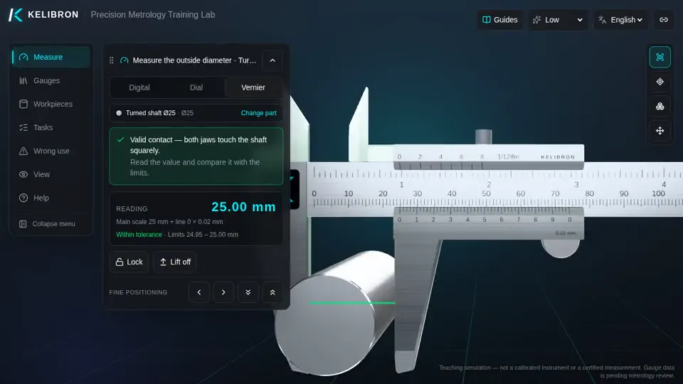
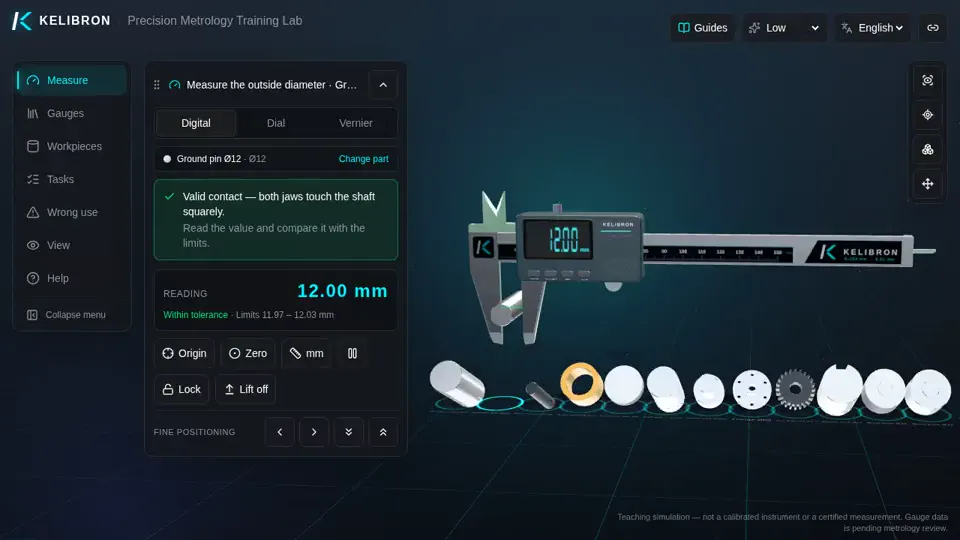
The lab’s vernier caliper reads to 0.02 mm, the same resolution as the NPL example, and its digital caliper to 0.01 mm, which gives 0.01/√12 = 0.003 mm for the resolution line. The lab does not yet scatter repeated readings: placing the caliper again at the same spot gives the same value, so the repeatability line has to come from real measurements until repeated-measurement practice is added.
References
- D. Flack, Callipers and Micrometers, NPL Measurement Good Practice Guide No. 40, Issue 2, 2014 (first issued 2001) · National Physical Laboratory
- JCGM 100:2008 — Evaluation of measurement data — Guide to the expression of uncertainty in measurement (GUM) · JCGM / BIPM
- ISO 13385-1:2019 — Geometrical product specifications (GPS) — Dimensional measuring equipment — Part 1: Design and metrological characteristics of callipers · ISO
- JCGM 200:2012 — International vocabulary of metrology — Basic and general concepts and associated terms (VIM, 3rd edition) · JCGM / BIPM
How the guides are checked against these sources: About KELIBRON.
Watch it done
Watch in the lab → Follow step by step →
Played back in the lab from domain commands; the reading and verdict come from the measurement model.
Practise in the lab

Questions
What goes into a caliper uncertainty budget?
Repeatability, resolution, flatness and parallelism of the measuring faces, and the calibration error or specification of the caliper; NPL GPG 40 lists these for its worked example.
How do you include resolution in an uncertainty budget?
Divide the resolution by √12: 0.02 mm gives 0.006 mm, 0.01 mm gives 0.003 mm.
Do I need k = 2.87 with five readings?
NPL’s guide suggests it as a simple, cautious choice: 2.87 is the t-factor for 4 degrees of freedom. The GUM’s Welch–Satterthwaite method gives about 33 effective degrees of freedom for this budget and k ≈ 2.08, because the Type B lines dominate.
Try it yourself
Open the same setup in the 3D lab and take the reading yourself.
Related guides
 Tolerances and decisionsMeasurement uncertainty basicsError is the measured value minus a reference value (VIM 2.16); uncertainty is a non-negative parameter characterizing the dispersion of the quantity values being attributed to a measurand, based on the information used (VIM 2.26).
 Tolerances and decisionsGauge R&R and measurement system analysis (MSA)Measurement system analysis (MSA) asks whether a measurement process is good enough for the decision made with it.
- Measuring methodsRadial and axial runout with a dial indicatorRunout is measured by turning the part one full revolution under a dial indicator: the runout value is the largest reading minus the smallest.